The Graph Indexer Office Hours #170

TL;DR: Derek from Data Nexus demos his PostgreSQL setup, including identifying and resolving query performance issues and practical tips for improving query performance.

Opening remarks

Hello everyone, and welcome to episode 170 of Indexer Office Hours!

GRTiQ 181

Catch the GRTiQ Podcast with Danny Zuckerman, co-founder at 3Box Labs, the web3 studio behind Ceramic Network. Ceramic is a decentralized database layer for web3 applications.

Join GRTiQ as Danny shares his journey, his thoughts on The Graph, and how it fits into the future of web3 data.

Repo watch

The latest updates to important repositories

Execution Layer Clients

• Geth New release v1.14.8 :
  • This is a maintenance release with bug fixes only.
• Arbitrum-nitro New release v3.1.1-beta.2 :
  • This release introduces support for fast confirmation, improves Anytrust DAS stability, adds new metrics, enhances tracing support, and includes important fixes such as correcting metrics typos, fixing reorg issues on init flags, and resolving a bug related to block hash retrieval in PopulateFeedBacklog.

Consensus Layer Clients

Information on the different clients can be found here.

• Teku: New release v24.8.0 :
  • This optional update addresses a startup failure bug in Teku 24.6.0 affecting machines with directly assigned public IP addresses, and includes a fix for the issue; no breaking changes are introduced, but the next release will require Java 21 and include changes to metrics.
• Lighthouse: New release v5.3.0 :
  • This medium-priority release includes performance optimizations, important bug fixes, new features, and several breaking changes, including a database schema upgrade for faster beacon node startup and more reliable block proposals with the new v3 block production API.

Protocol watch

The latest updates on important changes to the protocol

Forum Governance

• GIP-0067: Deprecate the L1 (mainnet) protocol

Contracts Repository

• fix: subgraphService access controll (OZ C-04) #990 (open)
• fix: add subgraph service as a caller when collecting from curation contract (OZ C-03) #989 (open)
• fix: addToDelegationPool access control and token transfer (OZ C-01 and C-02) (open)

Open discussion

• Derek from Data Nexus shares a PostgreSQL setup demo

Abel: We’ve got Derek here, who’s going to tell us all about his PostgreSQL setup. We had a very interesting conversation last week, and there was a lot of follow-up. One request was for this particular session, so Derek, the mic is yours.

Introduction

Derek:

Thanks. Let me share my screen. To give a quick backstory, before joining The Graph, I worked as a database administrator within the Microsoft SQL stack. All of the normal tools that I was used to went away. As I became more familiar with PostgreSQL, writing queries is mostly the same, but the underlying system tables and monitoring tools have changed.

It’s been kind of a fun experience to learn this type of stuff, but it is a little bit of figuring out: what is going to be the most workable? And, especially as an indexer, figuring out what matters and what doesn’t in terms of what’s going to make a noticeable difference on my bottom line.

Identifying Profitable Subgraphs 8:00

These are some of the things we started to do at Data Nexus, in terms of identifying which subgraphs we should be allocated to, who’s actively querying the network, and where we can start seeing query fee revenue make a difference. I’ve mentioned this a lot on other IOH calls, but we’ll drop 1,000 GRT allocations on pretty much anything that we can see that is producing some query traffic. Because if it’s making even 10 GRT in query fees per day, by the end of the month, you spend 30 cents opening and closing an allocation in bad times, and you might make a couple of dollars or whatever, and so it’s profitable to do that, but also you properly support consumers in the protocol and help them as they grow their applications.

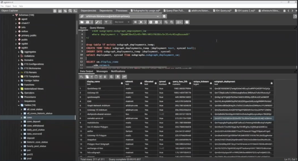
Example Query 9:10

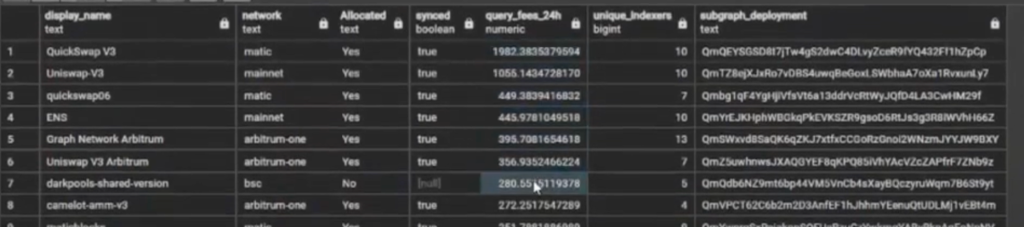
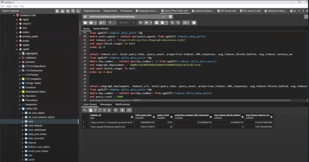
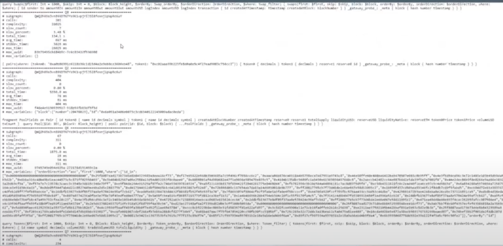
I’ll show you just one query that I put together. This one uses the quality of service subgraph, and it’s just looking at yesterday’s data points. Then I joined a bunch of other local tables to see if we are synced on it and if we are allocated to it in order to get some basic information.  So this is looking at yesterday’s data to figure out: Which subgraphs have the most traffic? Are we allocated to that subgraph? Are we even synced on that subgraph? How many queries are on it? How many other indexers are on it?

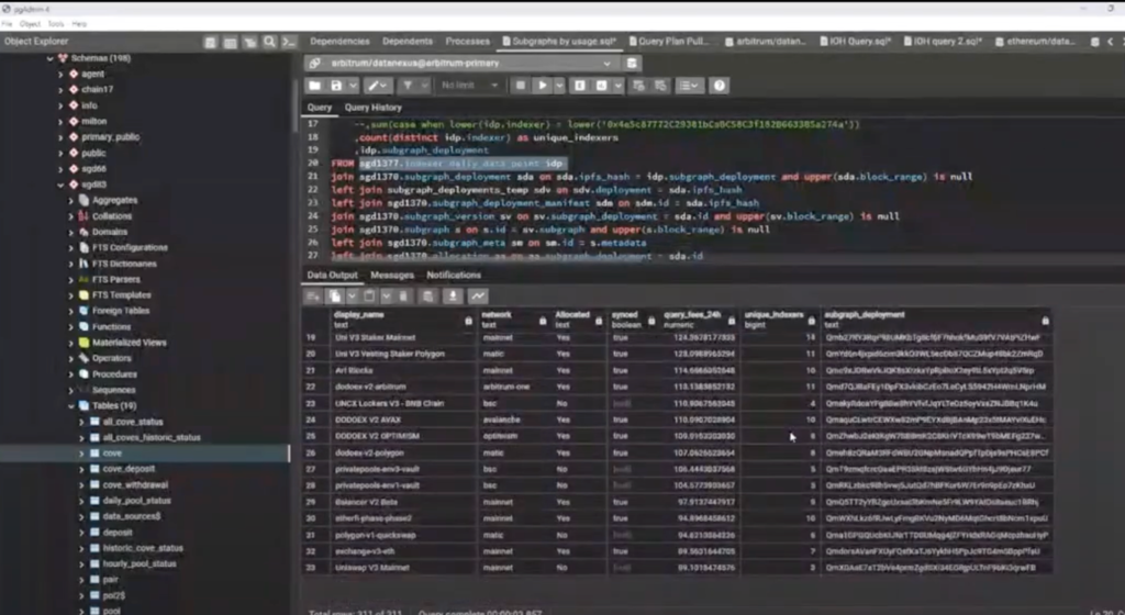
Like, sometimes we’ll scroll through this list and see that there’s only one other indexer. Okay, that’s probably the upgrade indexer. We can outperform them pretty easily. We should be able to take a lion’s share of whatever this amount is. So we’ll look through this list and this kind of drives which subgraphs we want to start syncing purely from a query fee mentality. Now 90-95% of our total stake is allocated with indexing rewards in mind, but the other 5-10% is allocated with query fees. So this is what kind of starts the process of allocating to some of these.

Question from the chat (10:31): The amount of queries I assume is in GRT, not in qty, right?

Derek:

Yes, correct. So this is GRT spent by all consumers. Like, in Uniswap’s case, this 1,000 GRT on this one subgraph: that might be Uniswap, that might be other people, no real clue, it just means that there was 1,055 GRT spent on queries for this one deployment, and it was split amongst these 10 indexers.

PostgreSQL Optimization Tips 11:11

So this is one thing that we’ve started to do because the easiest way to immediately increase your query traffic is to allocate on subgraphs that have queries. From there, we can start looking at tuning our database and tuning things, to help be more competitive against these other indexers. So this is kind of a workshop of: what does that next phase look like for someone who’s not really Postgres savvy or not really database savvy. What do we do here?

One of the first things I recommend is to go through this tutorial because the out-of-the-box Postgres solution is not set up for what we’re doing. It has very low default memory parameters. If you go through this tutorial, it’ll give you kind of the formula of saying this value should be 15 to 25% of your machine’s total RAM. Just go through the whole list. There’s some of them, one might be shared buffers, that are just stupidly low. There are certain things in there where just by increasing them, you’ll immediately start to see better performance across all subgraphs.

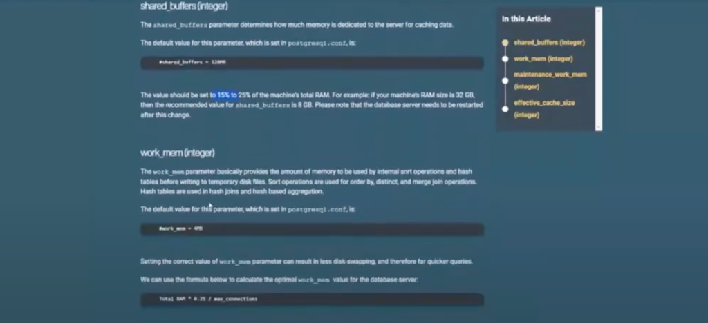
On our side, we’ve deviated a little bit from time to time on some of these values, but with no real noticeable success, and we’ve come back to this list and just said, okay, we’re just going to stick with this. Then we’ll start doing individual tweaks and tunes.

Query Optimization Example 13:23

So assuming that you are allocated to subgraphs that are producing queries and you’ve gone through and set up your basic configuration following this list, but you’re still getting poor latency, there’s a ton of reasons why that could be. It’s really unfortunate but this is kind of the role of a DBA to look in here and see what the heck is happening with all this data.

Together we can look through one of these.

I’m using pgAdmin to interface with my database. You just create a connection string and it’s really nice for being able to write queries, store multiple queries, and all that stuff. So, if you’re working out of the terminal, it’s not quite as user-friendly.

So we’re looking at this deployment, which I think is Uniswap Base deployment.

Database Sharding 14:49

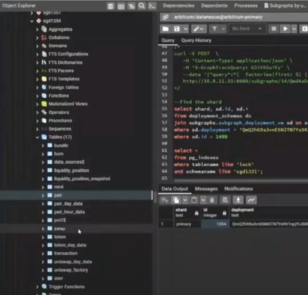
We will be working on our primary shard with subgraph number 1354. I know that in last week’s IOH we talked a little bit about sharding. And we do have a sharded database. I wouldn’t say that it’s set up the way that I really want it to be.

For example, on our primary shard, we’ve got a bunch of deployments on there. You know, Lutter mentioned you should probably just keep metadata and all that type of stuff.

The reason being, let’s say we have a Base subgraph that we’re syncing, we shove that onto our Base shard, a query comes in. That query is going to start at primary and it’s going to need to make a connection there before it realizes: okay, time to go to Base, let’s query there.  If you also have a bunch of subgraphs that are stored on your primary, you’re going to congest a lot of traffic into one place, and that can then prevent other shards from receiving their pass through quickly enough.

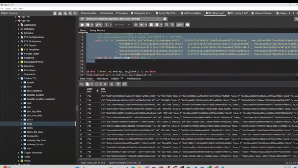
So we’re going to our primary shard and we’re looking for subgraph ID 1354. Inside the subgraph, we have all of our tables. And this is just a standard DEX.

DEX Indexing Improvements 16:40

You’ll pretty quickly learn that most DEXes have some easy improvements that you can add across the board, just because they’re all built in a very similar structure. Even their entity names are very similar because a lot of people start with the Uniswap V2 or Uniswap V3 contracts. Then they grab their subgraph, they fork that, and they add some of their own changes, but they usually keep the entity names the same, and they usually do the same things.

So this is the subgraph that we’re looking at. Just to get a general idea of the data that we have in here, we’ve got basic transactions like burn, mint, and swap—those are the things that users do.

Query posted in chat:

select count(*) from sgdNNN.table;

(gives you total records in the table)

You have tokens such as GRT and wrapped Ether, and all those things, you have pairs instead of pools because this is a Uniswap V2 contract, but pairs and pools are essentially the same thing. And then you have some time series data, to see what happened with a pair over a day’s time. Also liquidity position information.

I just happen to know that Uniswap on Base had a whole bunch of transactions over the past four or five months. When memecoins on Base started going crazy, they had a ton of interactions. We can just see inside of swap, we’ve got 13 million swaps that have happened on Uniswap V2. So that gives us kind of an idea of how much data we’re storing here.

Entities vs. Versions 19:43

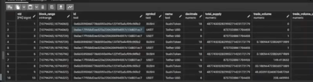
Keep in mind the way that we’re storing information with Graph Node. We’re storing full archival information, so you have this notion between entities and versions. It’s very evident when you get to the Token table, the difference between an entity and a version. Entities have the same ID, but a version is a singular record in the database. So, this entity for USDT is going to have some information about it, and that information is valid between this block range.

So, if you want to do some of our time-traveling queries, you’d be able to say: hey, my block is in this section. So you’ll have the instance where you have many versions for one entity and this is an easy optimization for that.

So I grabbed this query, and looking at the quality of service subgraph, I notice they are producing query traffic, and I’m not getting any of it, and our latency was quite bad.

Finding Troublesome Queries 21:07

Vincent set something up for us where we can pull the query logs. This is something from inside Graph Node. He set up an API so that I can go through and then scroll, and find out: here’s the GraphQL query, and these are the parameters that they put into that query. This is something that the website’s sending. So now I can see what queries are we receiving? It also gives us some basic information on how many times are we getting it? What’s the complexity of it? What’s my average time to resolve this query?

Like this one’s 7 seconds. That’s not good. But then you might have another one where it’s 600 milliseconds. Less than a second. That’s probably not going to be the problem. Then you can start to see, where are my problem children? If you’ve only got four queries for that subgraph, this is probably not one that you’ll want to optimize. But some of the higher volume ones, obviously you will.

So this is one that I took just because my average response time on it is 31 seconds.

Translating GraphQL to SQL 22:20

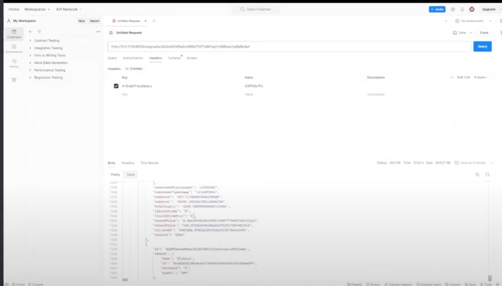
I want to see why this is taking so long. Unfortunately, I can’t just copy this GraphQL query into Postgres and execute it here because this is SQL, not GraphQL. The first thing that I have to do is to translate it into SQL.

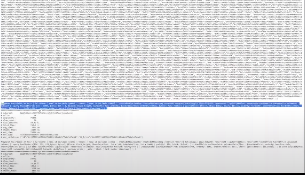
The way that you can do that is you just have to query your own node. Then you want to add a little header and you create a trace query. Add whatever your token is, and then when you run the query, at the bottom of your query you’ll get this trace. It’ll show you the SQL queries that were run in order to provide the results for your GraphQL query.

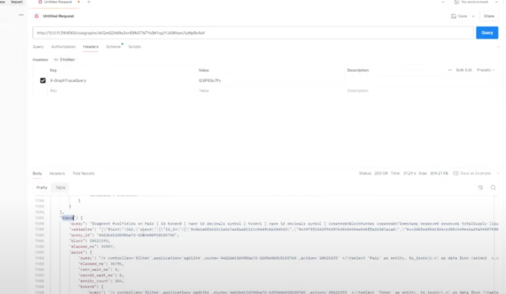
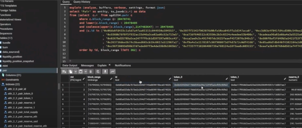
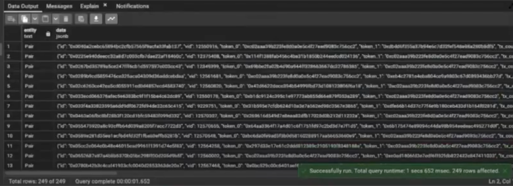
So we can see here this is one of the queries. I’ll typically just copy that and paste it into Postgres. It’s pretty raw when you receive it, so let me do it inside Postgres, it’s formatted slightly better.

So we’re going to select “pair” as an entity, as data. It’s going to be from this selection of data, and then we get all these little backslash t’s and all that stuff. So I manually go in here. There’s probably a better way to parse this.

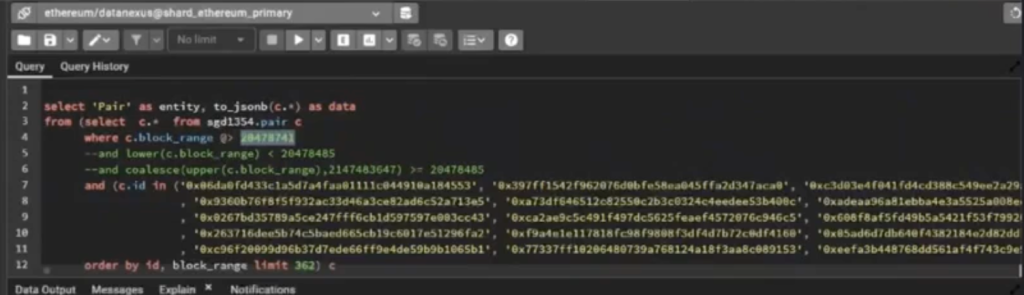
So here’s what the query looks like and the block number that it’s specifically querying is this one. So remember when we had that notion of versions and entities? It’s saying, give me all of the pairs where the ID is one of these 362 IDs, and do it specifically for this block number.

This is not that complex of a query. But remember this pair table. Because we had 12 million swaps, even if there are only 3,000 pools or 3,000 pairs, it’s going to have 12 million records, because it creates a new version every time a swap occurs. The total volume for that pair changed, the price changed, all these different data points changed, and now you have a new version of the same entity. So that’s how you can have lots of records for something that you should only have a few entities for.

Question from chat (26:00):

How much time would you say you spend optimizing for query performance compared to optimizing allocation selection and size?

Derek:

For allocation selection, we’ve got different dashboards and stuff that show the same thing that I just pulled up inside of pgAdmin. Mike will open and close our allocations and add new things that we should start syncing.

I spend probably three hours a week on query optimization. I’d love to spend all my time doing this because I really enjoy it. I find it to be a lot of fun because each time it’s like a puzzle. But at the same time, I can’t spend 40 hours a week trying to improve Data Nexus’s income by $400. If it means the difference of getting an extra $5,000 this month, that’s a different story than $500, so it’s something that we’ve been toying with a little bit.

Finding the Trace 27:08

So I’m looking at this query specifically, to run this inside my database. This is the same query that I just sent to my own Graph Node inside of Postman. I grab the trace. This is one of the steps of that query.

I’m going to go back to the trace. So we can see this is one step. And this one’s taking up a lot of the time. These two queries are sub selections, so they’re trying to get token information. It’s probably the token symbol, decimals, the address, all that type of stuff. These are relatively smaller so let’s start with this one and see what we can do.

Question: Why is that thing 7,000 lines of code? What else is inside that result?

Derek:

That’s the actual response to the query, so it’s got all the pair data that they’re selecting.

So running this query took 21 seconds just directly against my database, which is very bad. So this is the thing that I want to optimize.

Generate an Execution Plan 28:50

You can pull an execution plan, which will look like this:

explain (analyze, buffers, verbose, settings, format json)

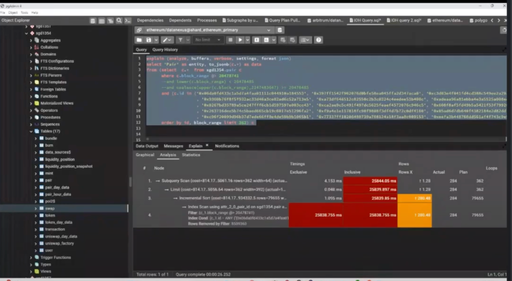
It might take another 20 seconds inside the database when you run a query. Postgres is going to try to figure out what’s the smartest way to execute this query.

It’s going to look at things like: What indexes exist on the table? What statistics do I know about this table? What do I think is going to be the smartest way to perform this query? A lot of the time, it does a very good job, but there are times where it does a terrible job just because it’s missing some information. Or so many new records have been inserted and it hasn’t reanalyzed what’s inside the table, etc. Typically, if your table’s only a thousand records or a million records, it’s not going to be that bad.

But once you start getting into the tens of millions, hundreds of millions, or greater, that’s where you’re going to start to see major scaling issues. You’re going to need to make sure that you’ve got proper indexing and proper statistics in place in order to tell your query planner: hey, you could spend a lot of time doing an inefficient query, or if you use these tools, you can start to do some smart things.

Here it’s showing that it’s trying to utilize this specific index, pair ID. So it’s trying to use this index, and it’s saying, yeah, it’s going to take a while.

Execution Plan Settings 30:25

Question: So in order to trigger that you have to run explain, analyze…? And how did you choose the options? Like, what does buffers do?

Derek:

It gives you some more information. You can literally add it before any select statement, and it will give you the execution plan. So now you’re seeing how Postgres thinks that I should execute this thing.

We have a membership with pgMustard. You can paste that same execution plan. I think they give you five for free. After you’ve read a few execution plans, it starts to make more sense.

We can see that when I first ran this it took about 100 seconds. When we just ran, it was down to 20 seconds. That was definitely an improvement. We can see that most of these steps in the execution plan are pretty simple.

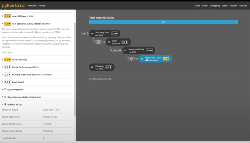
It’s this one that is our problem. So it wants to scan this whole index, and that’s taking a while. And the big issue that we’ll be able to see, is it thinks that it needs 46 gigabytes worth of memory to be able to read through that entire index, which is not good.

In actuality, it needs far less because it’s planning for a lot more rows than it actually needs to have. So I saw this, and I was immediately like, oh, this one is not so happy.

Generating Graphman Stats 32:24

So I asked Vincent, “Hey, can you run that Graph Node command?” to get the versions and entities.

graphman stats show sgd1499

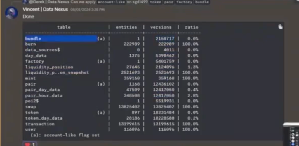
It gives us a table to be able to see how many entities something has, versus how many versions it has. You can see “bundle,” which just stores the price of Ether, and that’s used as a control to be able to figure out the price of other things. And it literally is just one entity. It just has a new version every time the price of anything changes.

You also have “pair,” which is the one that we’re working with, where they have a thousand different pairs, and they’ve got 12 million different versions.

“Swaps,” you have 13 million swaps where each swap is its own entity. And the data of that swap never changes. So in this one, you should have an exact parity between entities and versions, which would give you 100% here. And if this is ever true, the subgraph developer should have put an immutable entity here, because the data literally never changes. “Transaction,” the data never changes, “user,” the data never changes. Whether or not they did that is kind of outside of our control as indexers. But it’s something that we can complain about.

Using the account-like Flag 34:19

In our case, we’re dealing with pairs. We can see there are very few entities compared to the number of versions. My understanding from Lutter is we have the ability to set this flag for account-like.

That’s going to be especially useful in scenarios where you have a very low number of entities and a very high number of versions. So inside here, we’ve got 1100 entities and a whole bunch of versions. Let’s apply account-like. That should change the way that your query gets executed, slightly.

So, with this “contains” operator, we’ve got this block range that has two values in it. I want to make sure that the record that I’m selecting is true for this specific block, and we use the “contains” operator to obtain that. This can be very performant when you have a low number of records, but when you start having lots of records, it gets to be kind of heavy, and the index on that column gets to be kind of heavy.

Optimizing Queries 36:43

You can change it to these two things:

and lower(c.block_range) < 20478485

and coalesce(upper(c.block_range), 2147483647) >= 20478485

To break down what coalesce does, it’s going to select the first non-null value. So if this has a value, go ahead and select that. Otherwise, we’re going to use this number (2147483647), which is a magic number. It’s the largest value that a 32-byte integer can have. So you couldn’t store that number inside of this field. So it’s going to say where the lower block range value is less than this amount, and the upper block range value is greater than or equal to this amount.

Remember when we first ran that query, it took about 20 seconds. If we run it again using these, it now runs in 700 milliseconds, which is happy days for me.

One second or 1.6 seconds is not stellar, but it’s not terrible. Usually, you have your first run, which is the slow one, and then after things start to get stored inside of the cache, the cache will help speed things up. You have your index that’s already in cache, so you don’t need to re-pull it in there.

So when I ran this, I thought the first thing that we should do on this table is apply that account-like flag.

I started putting together queries, just to figure out if I can identify ahead of time the scenarios where we’ve got a really low number of entities and a really high number of versions, just so that we can proactively apply this flag. So far, we’ve got some mixed performance with that.

This is something where you need almost no skills. You just have to find a bulky table with a very low number of different records. It just has a bunch of versions, so you can go and apply this account-like flag and that should improve your query performance.

Once you run the graphman stats, and you notice that number is way bigger than this number, turn on account-like, then you’re good to go.

Turning Off the account-like Flag

Question: How do you revert if you accidentally set something on account-like ?

Vincent included in the chat the unset account-like flag:

graphman stats account-like sgd1354 pair -c

So you can you can test it out before you add it in there. So literally without any kind of index set prior to this, you just set it to account-like and it magically works faster.

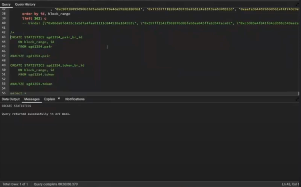
Creating Statistics 44:04

So the next thing that I want to do is I want to add some statistics, and there’s a command to do that from inside Graph Node.

Vincent can pop that into the chat:

CREATE STATISTICS sgd1354_pair_br_id

ON block_range, id

FROM sgd1354.pair

Statistics give the query planner a better gauge to see information types and values. It makes a histogram of data sampling. So it’s going to grab a certain percentage of the records and see how many times do the values start with the letter Q, the letter P, and the letter T. From there, it can start to be a little bit more intelligent. Let’s say I were to try to filter my query by a word that starts with the letter Z. It can probably jump straight towards the end of a certain index. It gives more information so we’re being more helpful to Postgres.

The downside of creating statistics is that it does use up more memory, so you don’t want to just go statistics-heavy and create them on everything.

You want to create statistics on the things that actually matter, and ideally, you can do it on columns that have what we call cardinality, where if one thing is increasing, the other thing is increasing in a similar way. Like a block number and a timestamp: those two increase together.

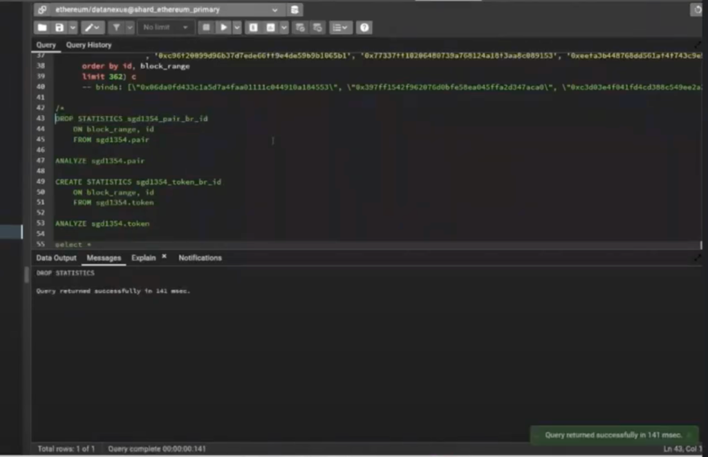
Remove Statistics

Question: How do I unset the statistics after I turn it on?

Derek:

From inside SQL, you just write drop statistics.

The word “drop” is always a little scary. You want to be really careful executing this in the terminal.

Okay, cool, so now we’ve got statistics. I’m hoping that things will have refreshed over here.

The first one took 15 seconds. That’s still not super happy. The other one took 1.3 seconds, which is a lot better.

Looking at some of the other indexers on this specific query: 400 milliseconds? I’ll take that all day long. Before I optimized, my average latency was 6,000 milliseconds or 6 seconds. If I can start to improve these queries, then I can get myself down closer to these numbers.

The downside is, that’s just one query. We have other queries that we can optimize as well, and the ones with not a lot of traffic I’m not going to spend time doing. If I find something that represents 90% of the traffic, and it’s slow, then that’s a prime one to look into.

The next step is how to start creating custom indexes.

There’s a great 30-minute video where someone goes through a B-tree index. I super recommend watching that because it’ll help explain why indexes speed up queries.

Derek finished the presentation with an example of an index. See the example and how it relates to optimizing an indexer on The Graph at 49:20.